
Hope to add bits of mathematics or mathematical news I find interesting.

Friday, January 1, 2016

Tuesday, December 15, 2015
Thursday, December 3, 2015
Wednesday, November 25, 2015
Thursday, November 19, 2015
On a class of random walks
I heard of these random walks from my number-theorist colleague Andrei Jorza who gave me a probabilistic translation of some observations in number theory. What follows is rather a variation on that theme.
There is a whole family of such walks, parametrized by a complex number $\newcommand{\ii}{\boldsymbol{i}}$ $\rho=\cos \theta +\ii \sin\theta$, $\theta\in [0,\pi]$, $\ii=\sqrt{-1}$.
This is discrete time walk on the configuration space $\newcommand{\lan}{\langle}$ $\newcommand{\ran}{\rangle}$
$$ \eC_\rho:= L[\rho] \times C(\rho,-\rho), $$
where $C(\rho,-\rho)$ is the subgroup of $S^1$ generated by $\pm\rho$, i.e.,
$$ C(\rho,-\rho)=\bigl\{\; \pm \rho^k;\;\;k\in\bZ \;\bigr\},$$
and $L[\rho]\subset \bC$ is the additive subgroup of $\bC$ generated by the elements $\rho^n$, $n\in\bZ_{\geq 0}$.
The state of the walk at time $n$ is given by a pair of random variables $(X_n, V_n)$, where one should think of $X_n\in L[\rho]$ as describing the "position'' and $V_n\in G(\rho,-\rho)$ as describing the ``velocity'' at time $n$.
Here is how the random walk takes place. Suppose that at time $n$ we are in the configuration $(X_n, V_n)$. To decide where to go next, toss a fair coin. If a the Head shows up then
$$V_{n+1}=\rho V_n,\;\; X_{n+1}= X_n+V_{n+1}. $$
Otherwise,
$$ V_{n+1}=-\rho V_n,\;\; X_{n+1}= X_n+V_{n+1}. $$
More abstractly, we are given a probability space $(\Omega,\eF,\bP)$ and a sequence of independent, identically distributed variables
$$ S_n:\Omega\to\{-1,1\},\;\;\bP[S_n=\pm 1]=\frac{1}{2},\;\;n\in\bZ_{\geq 0}. $$
If we set
$$
\whS_n:=\prod_{k=1}^nS_k, $$
then we have
$$
V_n= \whS_n \rho^n,\;\;X_n=\sum_{k=1}^n V_n=\sum_{k=1}^n \whS_k\rho_k.
$$
Observing that
$$\bE[\whS_k]=0,\;\;\var[\whS_k]=\prod_{j=1}^k\var[S_j]=1, $$ we deduce
$$\bE[X_n]=0,\;\;\var[S_n]=\bE[X_n\bar{X}_n] $$
$$=\sum_{j,k=1}^n \bE[ \whS_j\whS_k]\rho^{k-j}=\sum_{j=1}^n \bE[ \whS_j^2]+2\sum_{1\leq j<k\leq}^n \bE[ \whS_j\whS_k]\rho^{k-j}=n. $$
Example 1. Suppose that $\theta=\frac{\pi}{2}$ so that $\rho=\ii$. In this case $L[\rho]$ is the lattice $\bZ^2\subset \bC$ and $G(\ii,-\ii)$ is the group of forth order roots of $1$. At time $n=0$, the moving particle is at the origin facing East,. turns right or left (in this case North/South) with equal probability. Once reaches a new intersection, it turns right/left with equal probability. The following MAPLE generated animation a loop describes a 90-step portion of one such walk.

This is somewhat typical of what one observes in general.
Example 2. Suppose that $\theta =\frac{\pi}{3}$. In this case $G(\rho,-\rho)$ is the group of 6th order roots of $1$ and $L[\rho]$ is a lattice in $\bC$. The following MAPLE generated animation depicts a 90 step portion of such a walk and the patterns you observe are typical.

Example 3. Assume that the angle $\theta$ is small and $\frac{\theta}{\pi}$ is not rational, say $\cos \theta=0.95$. The animation below depicts a 90-step stretch of such a walk.

Example 4. For comparison, I have included an animation of a 90-step segment of the usual uniform random walk on $\bZ^2$.
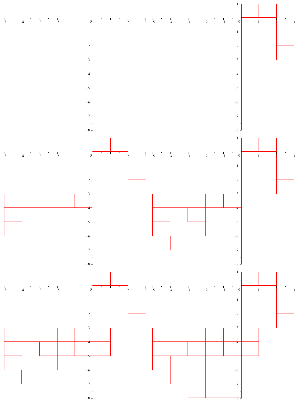
Clearly, I am interested to figure out what is happening and I have a hard time asking a good question. A first question that comes to my mind would be to find statistical invariants that would distinguish the random walk in Example 1 from the random walk in Example 4. I will refer to them as $RW_1$ and $RW_4$
Clear each of these two walks surround many unit squares with vertices in the lattice $\bZ^2$. For $j=1,4$ will denote by $s_j(n)$ the expected number of unit squares surrounded by a walk of $RW_j$ of length $n$.. Which grows faster as $n\to\infty$, $s_1(n)$ or $s_4(n)$?
I will probably update this posting as I get more ideas, but maybe this shot in the dark will initiate a conversation and will suggest other, better questions.
Sunday, November 15, 2015
Tuesday, November 10, 2015
Random subdivisions of an interval
This is a classical problem, but I find it very appealing.
Drop $n$ points $X_1,\dotsc, X_n$ at random in the unit interval, uniformly and independently. These points divide the interval into $n+1$ sub-intervals. Their lengths are called the spacings of the subdivision. What is the expected length of the longest of these intervals? What is its asymptotic behavior for $n$ large?
I was surprised to find out that the problem of finding the expectation of the largest segment was solved in late 19th century. What follows is a more detailed presentation of the arguments in Sec. 6.3 of the book Order Statistics by H.A. David and H.N. Nagaraja.
If you read French, you can click here to see what P. Levy had to say about this problem back in 1939.
Relabel by $Y_1,\dotsc, Y_n$, the points $\{X_1,\dotsc, X_n\}\subset [0,1]$ so that $Y_1\leq \cdots \leq Y_n$. We set
$$ Y_0=0,\;\;Y_{n+1}=1,\;\;\;\;L_n= \max_{1\leq i\leq n+1} Y_i-Y_{i-1},.$$
We want to determine the expectation $\newcommand{\bE}{\mathbb{E}}$ $E_n$ of $L_n$.
The probability distribution of $\vec{X}=(X_1,\dotsc, X_n)$ $\newcommand{\bone}{\boldsymbol{1}}$ is
$$ p_{\vec{X}}(dx)=\bone_{C_n}(x_1,\dotsc, x_n) dx_1\cdots dx_n, \;\;C_n=[0,1]^n, $$
where $\bone_A$ denotes the indicator function of a subset $A$ of a given set $S$.
The probability distribution of $\vec{Y}=(Y_1,\dotsc, Y_n)$ is
$$p_{\vec{Y}}(dy)= n! \bone_{T_n}(y_1,\dotsc, y_n) dy_1\cdots dy_n, $$
where $T_n$ is the simplex $\newcommand{\bR}{\mathbb{R}}$
$$ T_n=\bigl\{ y\in\bR^n;\;\;0\leq y_1\leq \cdots \leq y_n\leq 1\,\bigr\}. $$
The spacings are the lengths of the $n+1$ segments that the points $Y_1,\dotsc, Y_n$ determine on $[0,1]$
$$ S_i= Y_{i}-Y_{i-1},\;\; i=1,\dotsc, n+1, $$
where $Y_{n+1}:=1$. The resulting map $\vec{Y}\to\vec{S}=\vec{S}(\vec{Y})$ induces a linear bijection
$$ T_n\to \Delta_n=\bigl\{\, (s_1,\dotsc, s_{n+1})\in\bR_{\geq 0}^{n+1};\;\;s_1+\cdots+s_{n+1}=1\,\bigr\}. $$
This shows that the probability density is $\DeclareMathOperator{\vol}{vol}$
$$p_{\vec{S}}(ds) =\frac{1}{\vol(\Delta_n)} dV_{\Delta_n}, $$
where $dV_{\Delta_n}$ denote the usual Euclidean volume density on the standard simplex $\Delta_n$. This description shows that the random vector of spacings $\vec{S}$ is exchangeable, i.e., the probability density of $\vec{S}$ is invariant under permutation of the components. Thus the joint probability distribution of any group of $k$ components of $\vec{S}$, $k\leq n$, is the same as the joint distribution of the first $k$-components $S_1,\dotsc, S_k$.
The joint probability distribution of the first $n$ components is
$$ p_n(ds)= n! \bone_{D_n}(s_1,\dotsc,s_n) ds, $$
where $D_n$ is the simplex
$$ D_n=\{\, (s_1,\dotsc, s_n)\in\bR^n_{\geq 0};\;\;s_1+\cdots +s_n\leq 1\,\}. $$
Indeed, $(S_1,\dotsc, S_n)\in D_n$ and
$$ ds=|ds_1\cdots ds_n|=|d y_1\wedge d(y_2-y_{1})\wedge \cdots \wedge d(y_{n}-y_{n-1})|=|dy_1\cdots d y_n|. $$
The joint density of the first $n-1$ components $(S_1, \dotsc, S_{n-1})$ is
$$ p_{n-1}(s_1,\dotsc, s_{n-1}) = n! \int_0^\infty \bone_{D_n}(s_1,\dotsc, s_n) ds_n $$
$$= n! \bone_{D_{n-1}}(s_1,\dotsc, s_{n-1})\int_0^{1-s+1-\cdots-s_{n-1}} ds_n= n! \bone_{D_{n-1}}(s_1,\dotsc, s_{n-1})(1-s_1-\cdots-s_{n-1}) $$
The joint density of the first $(n-2)$ components is
$$ p_{n-2}(s_1,\dots, s_{n-2})=\int_0^\infty p_{n-1}(s_1,\dotsc, s_{n-1}) ds_{n-1} $$
$$ = n!\bone_{D_{n-2}}(s_1,\dotsc, s_{n-2})\int_0^{1-s_1-\cdots-s_{n-2}} (1-s_1-\cdots -s_{n-1}) d s_{n-1} = \frac{n!}{2!} \bone_{D_{n-2}}(s_1,\dotsc, s_{n-2})(1-s_1-\cdots -s_{n-2})^2. $$
Iterating, we deduce that the joint probability density of the the first $k$ variables is
$$ p_k(s_1,\dotsc, s_k) =\frac{n!}{(n-k)!}p_{D_k}(s_1,\dotsc, s_k) (1-s_1-\cdots-s_k)^{n-k}. $$
If $1\leq k\leq n$, then$\newcommand{\bP}{\mathbb{P}}$
$$ \bP[S_1>s,\dotsc, S_k>s]=\frac{n!}{(n-k)!}\int_s^\infty\cdots\int_s^\infty p_{D_k}(s_1,\dotsc, s_k) (1-s_1-\cdots-s_k)^{n-k} ds_1\dotsc ds_k $$
$$=\frac{n!}{(n-k)!}\int_s^1ds_1\int_s^{1-s_1}ds_2\cdots\int_s^{1-s_1-\cdots-s_{k-1}} (1-s_1-\cdots-s_k)_+^{n-k} ds_k =(1-ks)_+^n,\;\;x_+:=\max(x,0).$$
Also
$$ \bP[S_1>s,\dotsc, S_n>s, S_{n+1}>s] = \bP[S_1>s,\dotsc, S_n>s, S_1+S_2+\cdots +S_n\leq 1-s]$$
$$=n!\int_{\substack{s_1,\dotsc s_{n}>s\\ s_1+\cdots +s_{n}\leq 1-s}}ds_1\cdots d s_{n} $$
$$=n!\int_{\substack{s_1,\dotsc s_{n-1}>s\\ s_1+\cdots +s_{n-1}\leq 1-2s}}ds_1\cdots d s_{n-1}\int_s^{1-s-s_1-\cdots -s_{n-1}} d s_n $$
$$= n!\int_{\substack{s_1,\dotsc s_{n-1}>s\\ s_1+\cdots +s_{n-1}\leq 1-2s}} (1-2s-s_1-\cdots -s_{n-1}) ds_1\cdots ds_{n-1} $$
$$=n!\int_{\substack{s_1,\dotsc s_{n-2}>s\\ s_1+\cdots +s_{n-2}\leq 1-3s}}ds_1\cdots ds_{n-2}\int_s^{1-2s-s_1-\cdots -s_{n-2}} (1-2s-s_1-\cdots -s_{n-1}) d s_{n-1} $$
$$=\frac{n!}{2!} \int_{\substack{s_1,\dotsc s_{n-2}>s\\ s_1+\cdots +s_{n-2}\leq 1-3s}} (1-3s-s_1-\cdots -s_{n-2})^2 ds_1\cdots ds_{n-2} $$
$$ =\frac{n!}{2!} \int_{\substack{s_1,\dotsc s_{n-3}>s\\ s_1+\cdots +s_{n-3}\leq 1-4s}} ds_1\cdots ds_{n-3} \int_s^{1-3s -s_1-\cdots -s_{n-3}} (1-3s-s_1-\cdots -s_{n-2})^2ds_{n-2}$$
$$=\frac{n!}{3!} \int_{\substack{s_1,\dotsc s_{n-3}>s\\ s_1+\cdots +s_{n-3}\leq 1-4s}} (1-4s-s_1-\cdots -s_{n-3})^3ds_1\cdots ds_{n-3} $$
$$=\cdots = \bigl(\, 1-(n+1)s\,\bigr)_+^n. $$
With
$$ L_n:=\max_{1\leq i\leq n+1} S_i $$
we have
$$\bP[L_n>s]=\bP\left[\,\bigcup_{i=1}^{n+1}\bigl\lbrace\, S_i>s\,\bigr\rbrace\,\right] $$
(use inclusion-exclusion exchangeability)
$$ = \sum_{k=1}^{n+1}(-1)^{k+1}\binom{n+1}{k} \bP\bigl[\, S_1>s,\dotsc, S_k>s\,\bigr] =\sum_{k=1}^{n+1} \binom{n+1}{k}(1-ks)_+^n .$$
The last equality is sometime known as Whitworth formula and it goes all the way back to 1897. We have
$$ E_n=\bE[L_n]=\int_0^\infty \bP[L_n>s] ds =\sum_{k=1}^{n+1}(-1)^{k+1} \binom{n+1}{k}\int_0^\infty (1-ks)_+^n ds = \sum_{k=1}^{n+1}(-1)^{k+1} \binom{n+1}{k}\int_0^{1/k}(1-ks)^n ds $$
$$=\frac{1}{n+1} \sum_{k=1}^{n+1}(-1)^{k+1} \frac{1}{k} \binom{n+1}{k}=\sum_{k=1}^{n+1}(-1)^{k+1} \frac{1}{k^2} \binom{n}{k-1}. $$
Here is $E_n$ answers for small $n$ (thank you MAPLE)
$$ E_1=\frac{3}{4},\;\;E_2=\frac{11}{18},\;\;E_3=\frac{25}{48},\;\;E_4=\frac{137}{300},\;\; E_5=\frac{49}{120}. $$
It turn out that $L_n$ is highly concentrated around its mean. In the work of P. Levy I mentioned earlier he showed that the random variables $nL_n-\log n$ converges in probability to a random variable $X_\infty$ with probability distribution $\mu$ given by
$$ \mu\bigl(\,(-\infty,x])= \exp\bigl(\,-e^{-x}\,\bigr),\;\;x\geq 0.$$
Moreover
$$\lim_{n\to \infty} \bE[\, nL_n-\log n\,]=\gamma=\bE[X_\infty],\;\;\lim_{n\to \infty}\mathrm{Var}[ nL_n\,]=\frac{\pi^2}{6}=\mathrm{Var}[X_\infty]. $$
$$\frac{n}{\log n} L_n \to 1\;\; \mbox{a.s.} $$
Note that this shows that
$$E_n\sim\frac{\log n}{n}\;\; \mbox{as $n\to \infty$}. $$
I'll stop here, but you can learn more from this paper of Luc Devroye and its copious list of references.
Drop $n$ points $X_1,\dotsc, X_n$ at random in the unit interval, uniformly and independently. These points divide the interval into $n+1$ sub-intervals. Their lengths are called the spacings of the subdivision. What is the expected length of the longest of these intervals? What is its asymptotic behavior for $n$ large?
I was surprised to find out that the problem of finding the expectation of the largest segment was solved in late 19th century. What follows is a more detailed presentation of the arguments in Sec. 6.3 of the book Order Statistics by H.A. David and H.N. Nagaraja.
If you read French, you can click here to see what P. Levy had to say about this problem back in 1939.
Relabel by $Y_1,\dotsc, Y_n$, the points $\{X_1,\dotsc, X_n\}\subset [0,1]$ so that $Y_1\leq \cdots \leq Y_n$. We set
$$ Y_0=0,\;\;Y_{n+1}=1,\;\;\;\;L_n= \max_{1\leq i\leq n+1} Y_i-Y_{i-1},.$$
We want to determine the expectation $\newcommand{\bE}{\mathbb{E}}$ $E_n$ of $L_n$.
The probability distribution of $\vec{X}=(X_1,\dotsc, X_n)$ $\newcommand{\bone}{\boldsymbol{1}}$ is
$$ p_{\vec{X}}(dx)=\bone_{C_n}(x_1,\dotsc, x_n) dx_1\cdots dx_n, \;\;C_n=[0,1]^n, $$
where $\bone_A$ denotes the indicator function of a subset $A$ of a given set $S$.
The probability distribution of $\vec{Y}=(Y_1,\dotsc, Y_n)$ is
$$p_{\vec{Y}}(dy)= n! \bone_{T_n}(y_1,\dotsc, y_n) dy_1\cdots dy_n, $$
where $T_n$ is the simplex $\newcommand{\bR}{\mathbb{R}}$
$$ T_n=\bigl\{ y\in\bR^n;\;\;0\leq y_1\leq \cdots \leq y_n\leq 1\,\bigr\}. $$
The spacings are the lengths of the $n+1$ segments that the points $Y_1,\dotsc, Y_n$ determine on $[0,1]$
$$ S_i= Y_{i}-Y_{i-1},\;\; i=1,\dotsc, n+1, $$
where $Y_{n+1}:=1$. The resulting map $\vec{Y}\to\vec{S}=\vec{S}(\vec{Y})$ induces a linear bijection
$$ T_n\to \Delta_n=\bigl\{\, (s_1,\dotsc, s_{n+1})\in\bR_{\geq 0}^{n+1};\;\;s_1+\cdots+s_{n+1}=1\,\bigr\}. $$
This shows that the probability density is $\DeclareMathOperator{\vol}{vol}$
$$p_{\vec{S}}(ds) =\frac{1}{\vol(\Delta_n)} dV_{\Delta_n}, $$
where $dV_{\Delta_n}$ denote the usual Euclidean volume density on the standard simplex $\Delta_n$. This description shows that the random vector of spacings $\vec{S}$ is exchangeable, i.e., the probability density of $\vec{S}$ is invariant under permutation of the components. Thus the joint probability distribution of any group of $k$ components of $\vec{S}$, $k\leq n$, is the same as the joint distribution of the first $k$-components $S_1,\dotsc, S_k$.
The joint probability distribution of the first $n$ components is
$$ p_n(ds)= n! \bone_{D_n}(s_1,\dotsc,s_n) ds, $$
where $D_n$ is the simplex
$$ D_n=\{\, (s_1,\dotsc, s_n)\in\bR^n_{\geq 0};\;\;s_1+\cdots +s_n\leq 1\,\}. $$
Indeed, $(S_1,\dotsc, S_n)\in D_n$ and
$$ ds=|ds_1\cdots ds_n|=|d y_1\wedge d(y_2-y_{1})\wedge \cdots \wedge d(y_{n}-y_{n-1})|=|dy_1\cdots d y_n|. $$
The joint density of the first $n-1$ components $(S_1, \dotsc, S_{n-1})$ is
$$ p_{n-1}(s_1,\dotsc, s_{n-1}) = n! \int_0^\infty \bone_{D_n}(s_1,\dotsc, s_n) ds_n $$
$$= n! \bone_{D_{n-1}}(s_1,\dotsc, s_{n-1})\int_0^{1-s+1-\cdots-s_{n-1}} ds_n= n! \bone_{D_{n-1}}(s_1,\dotsc, s_{n-1})(1-s_1-\cdots-s_{n-1}) $$
The joint density of the first $(n-2)$ components is
$$ p_{n-2}(s_1,\dots, s_{n-2})=\int_0^\infty p_{n-1}(s_1,\dotsc, s_{n-1}) ds_{n-1} $$
$$ = n!\bone_{D_{n-2}}(s_1,\dotsc, s_{n-2})\int_0^{1-s_1-\cdots-s_{n-2}} (1-s_1-\cdots -s_{n-1}) d s_{n-1} = \frac{n!}{2!} \bone_{D_{n-2}}(s_1,\dotsc, s_{n-2})(1-s_1-\cdots -s_{n-2})^2. $$
Iterating, we deduce that the joint probability density of the the first $k$ variables is
$$ p_k(s_1,\dotsc, s_k) =\frac{n!}{(n-k)!}p_{D_k}(s_1,\dotsc, s_k) (1-s_1-\cdots-s_k)^{n-k}. $$
If $1\leq k\leq n$, then$\newcommand{\bP}{\mathbb{P}}$
$$ \bP[S_1>s,\dotsc, S_k>s]=\frac{n!}{(n-k)!}\int_s^\infty\cdots\int_s^\infty p_{D_k}(s_1,\dotsc, s_k) (1-s_1-\cdots-s_k)^{n-k} ds_1\dotsc ds_k $$
$$=\frac{n!}{(n-k)!}\int_s^1ds_1\int_s^{1-s_1}ds_2\cdots\int_s^{1-s_1-\cdots-s_{k-1}} (1-s_1-\cdots-s_k)_+^{n-k} ds_k =(1-ks)_+^n,\;\;x_+:=\max(x,0).$$
Also
$$ \bP[S_1>s,\dotsc, S_n>s, S_{n+1}>s] = \bP[S_1>s,\dotsc, S_n>s, S_1+S_2+\cdots +S_n\leq 1-s]$$
$$=n!\int_{\substack{s_1,\dotsc s_{n}>s\\ s_1+\cdots +s_{n}\leq 1-s}}ds_1\cdots d s_{n} $$
$$=n!\int_{\substack{s_1,\dotsc s_{n-1}>s\\ s_1+\cdots +s_{n-1}\leq 1-2s}}ds_1\cdots d s_{n-1}\int_s^{1-s-s_1-\cdots -s_{n-1}} d s_n $$
$$= n!\int_{\substack{s_1,\dotsc s_{n-1}>s\\ s_1+\cdots +s_{n-1}\leq 1-2s}} (1-2s-s_1-\cdots -s_{n-1}) ds_1\cdots ds_{n-1} $$
$$=n!\int_{\substack{s_1,\dotsc s_{n-2}>s\\ s_1+\cdots +s_{n-2}\leq 1-3s}}ds_1\cdots ds_{n-2}\int_s^{1-2s-s_1-\cdots -s_{n-2}} (1-2s-s_1-\cdots -s_{n-1}) d s_{n-1} $$
$$=\frac{n!}{2!} \int_{\substack{s_1,\dotsc s_{n-2}>s\\ s_1+\cdots +s_{n-2}\leq 1-3s}} (1-3s-s_1-\cdots -s_{n-2})^2 ds_1\cdots ds_{n-2} $$
$$ =\frac{n!}{2!} \int_{\substack{s_1,\dotsc s_{n-3}>s\\ s_1+\cdots +s_{n-3}\leq 1-4s}} ds_1\cdots ds_{n-3} \int_s^{1-3s -s_1-\cdots -s_{n-3}} (1-3s-s_1-\cdots -s_{n-2})^2ds_{n-2}$$
$$=\frac{n!}{3!} \int_{\substack{s_1,\dotsc s_{n-3}>s\\ s_1+\cdots +s_{n-3}\leq 1-4s}} (1-4s-s_1-\cdots -s_{n-3})^3ds_1\cdots ds_{n-3} $$
$$=\cdots = \bigl(\, 1-(n+1)s\,\bigr)_+^n. $$
With
$$ L_n:=\max_{1\leq i\leq n+1} S_i $$
we have
$$\bP[L_n>s]=\bP\left[\,\bigcup_{i=1}^{n+1}\bigl\lbrace\, S_i>s\,\bigr\rbrace\,\right] $$
(use inclusion-exclusion exchangeability)
$$ = \sum_{k=1}^{n+1}(-1)^{k+1}\binom{n+1}{k} \bP\bigl[\, S_1>s,\dotsc, S_k>s\,\bigr] =\sum_{k=1}^{n+1} \binom{n+1}{k}(1-ks)_+^n .$$
The last equality is sometime known as Whitworth formula and it goes all the way back to 1897. We have
$$ E_n=\bE[L_n]=\int_0^\infty \bP[L_n>s] ds =\sum_{k=1}^{n+1}(-1)^{k+1} \binom{n+1}{k}\int_0^\infty (1-ks)_+^n ds = \sum_{k=1}^{n+1}(-1)^{k+1} \binom{n+1}{k}\int_0^{1/k}(1-ks)^n ds $$
$$=\frac{1}{n+1} \sum_{k=1}^{n+1}(-1)^{k+1} \frac{1}{k} \binom{n+1}{k}=\sum_{k=1}^{n+1}(-1)^{k+1} \frac{1}{k^2} \binom{n}{k-1}. $$
Here is $E_n$ answers for small $n$ (thank you MAPLE)
$$ E_1=\frac{3}{4},\;\;E_2=\frac{11}{18},\;\;E_3=\frac{25}{48},\;\;E_4=\frac{137}{300},\;\; E_5=\frac{49}{120}. $$
It turn out that $L_n$ is highly concentrated around its mean. In the work of P. Levy I mentioned earlier he showed that the random variables $nL_n-\log n$ converges in probability to a random variable $X_\infty$ with probability distribution $\mu$ given by
$$ \mu\bigl(\,(-\infty,x])= \exp\bigl(\,-e^{-x}\,\bigr),\;\;x\geq 0.$$
Moreover
$$\lim_{n\to \infty} \bE[\, nL_n-\log n\,]=\gamma=\bE[X_\infty],\;\;\lim_{n\to \infty}\mathrm{Var}[ nL_n\,]=\frac{\pi^2}{6}=\mathrm{Var}[X_\infty]. $$
$$\frac{n}{\log n} L_n \to 1\;\; \mbox{a.s.} $$
Note that this shows that
$$E_n\sim\frac{\log n}{n}\;\; \mbox{as $n\to \infty$}. $$
I'll stop here, but you can learn more from this paper of Luc Devroye and its copious list of references.
Denote by $A_n$ the smallest spacing
$$ A_n:=\min_{1\leq k\leq n+1} S_k. $$.
Note that
$$\bP[ A_n>a]=\bP[ S_1,S_2,\dotsc, S_{n+1}>a]=\big( 1-(n+1)a\big)^n_+. $$
Hence
$$ \bE[ A_n]=\int_0^\infty\bP[A_n>a] da= \int_0^\infty \big( 1-(n+1)a\big)^n_+ da=\int_0^{\frac{1}{n+1}} (1-(n+1)a)^n da$$
$$ = \frac{1}{n+1}\int_0^1 (1-t)^n dt= \frac{1}{(n+1)^2}. $$
Saturday, November 7, 2015
The Luzin affair
I was not aware that Luzin was persecuted by Stalin and some of his detractors were big names like Kolmogorov and Sobolev.
"Aleksandrov, Kolmogorov and some other students of Luzin accused him of plagiarism and various forms of misconduct. Sergei Sobolev and Otto Schmidt incriminated him with charges of disloyalty to Soviet power. "
Nikolai Luzin - Wikipedia, the free encyclopedia
"Aleksandrov, Kolmogorov and some other students of Luzin accused him of plagiarism and various forms of misconduct. Sergei Sobolev and Otto Schmidt incriminated him with charges of disloyalty to Soviet power. "
Nikolai Luzin - Wikipedia, the free encyclopedia
Friday, October 23, 2015
Monday, October 19, 2015
Wednesday, October 7, 2015
Wednesday, September 9, 2015
Friday, February 20, 2015
Springer Verlag is one fucked-up company: the Alzheimer years. (Please repost)
In an earlier post I described my experience with Springer's new editing practices. Briefly, they're cheap SOBs. ( SOB:= sonovabitch) The saga continues.
Two days ago I received this nice letter from them, thanking me for my refereeing services. Part of the thank-you was an electronic discount token, good for two weeks that I can use to purchase one book of my choice at 50% discount.
The problem is that their shopping website is either not working, or I may be blacklisted. For several months I could not purchase anything there. That did not bother me too much because I could always go to the more reliable Amazon site. I cannot do this with my stupid token: I have to use it on their website which is reliably not working. My attempts to contact the customer service were fruitless (as I write this).
Here is a company that forgot how books are edited, cannot sell them on electronic platforms, and cannot handle customer inquires.
I was pissed off, but then I became worried: maybe one of world's largest media company is run by people suffering from early onset Alzheimer. This seems the most plausible explanation for a behavior displaying forgetfulness of the most basic business practices. Or maybe their just bumbling idiots in charge of the Titanic.
Two days ago I received this nice letter from them, thanking me for my refereeing services. Part of the thank-you was an electronic discount token, good for two weeks that I can use to purchase one book of my choice at 50% discount.
The problem is that their shopping website is either not working, or I may be blacklisted. For several months I could not purchase anything there. That did not bother me too much because I could always go to the more reliable Amazon site. I cannot do this with my stupid token: I have to use it on their website which is reliably not working. My attempts to contact the customer service were fruitless (as I write this).
Here is a company that forgot how books are edited, cannot sell them on electronic platforms, and cannot handle customer inquires.
I was pissed off, but then I became worried: maybe one of world's largest media company is run by people suffering from early onset Alzheimer. This seems the most plausible explanation for a behavior displaying forgetfulness of the most basic business practices. Or maybe their just bumbling idiots in charge of the Titanic.
Wednesday, November 26, 2014
Thursday, November 13, 2014
Wednesday, November 5, 2014
Friday, October 31, 2014
A new method of constructing connections on vector bundles
This post was suggested by a question on the MathOverflow site. After I answered part of it I noticed that it is related to a recent work of mine of a probabilistic nature. What follows involves no probability. $\newcommand{\bR}{\mathbb{R}}$ $\newcommand{\pa}{\partial}$ As far as the terminology concerning connections, I'll stick to the terminology in Section 3.3. of my book.
Suppose that $M$ is a smooth manifold of dimension $E\to M$ is a real, smooth vector bundle of rank $\nu$ over $M$. We define a pairing on $E$ to be a section of the bundle $E^*\boxtimes E^*\to M\times M$, where $E^*\boxtimes E^*$ is the vector bundle $\pi_1^* E^*\otimes \pi_2^*E^*$, $\pi_i(x_1,x_2)=x_i$, $\forall (x_1,x_2)\in M\times M$, $i=1,2$.
For $x,y\in M$ we can view $B_{x,y}\in E_x^*\times E^*_y$ as a bilinear map
$$ B_{x,y}: E_x\times E_y\to \bR. $$
This induces a linear map
$$ S_{x,y}= S(B)_{x,y}: E_y\to E^*_x. $$
We say that the pairing is nondegenerate if for any $x\in M$ the bilinear map $B(x,x): E_x\times E_x\to \bR $ is nondegenerate. In particular, this induces an isomorphism
$$S_x=S_{x,x}: E_x\to E^*_x.$$
We obtain tunneling operators
$$T(x,y)= S_x^{-1}S_{x,y}: E_y\to E_x. $$
Fix an open coordinate patch $\newcommand{\eO}{{\mathscr{O}}}$ $\eO\subset M$ with coordinates $(x^i)_{1\leq i\leq m}$. Assume $\eO$ is sufficiently small so $E$ trivializes over $\eO$. Suppose that $\newcommand{\be}{\boldsymbol{e}}$ $\underline{\be}(x)=(\be_\alpha(x))_{1\leq \alpha\leq \nu}$ is a local frame of $E$ over $\eO$. We denote by $\newcommand{\ur}{\underline{\mathbb{R}}}$ $\ur_\eO$ the trivial vector bundle $\bR^\nu\times \eO\to\eO$.
The local frame $\underline{\be}$ $\newcommand{\ube}{{\underline{\boldsymbol{e}}}}$ defines a bundle isomorphism $\Phi(\underline{\be}):\ur_\eO\to E_\eO$. In the local frame $\ube$ the tunelling are represented by$\DeclareMathOperator{\Endo}{End}$ $\DeclareMathOperator{\Aut}{Aut}$ a tunneling map
$$T_\ube:\eO\times \eO\to\Endo(\bR^\nu),\;\;T_\ube(x,y)= \Phi_x(\ube)^{-1}T(x,y)\Phi_y(\ube) . $$
Note that $T_\ube(x,x) = \mathbf{1}_{\bR^\nu}$. For $i=1,\dotsc, m$ define
$$\Gamma_i(\ube):\eO\to \Endo(\bR^\nu),\;\;\Gamma_i(\ube,x)=-\pa_{x^i}T_\ube(x,y)\bigl|_{y=x}. $$
We set
$$\Gamma(\ube,x)=\sum_{i=1}^m \Gamma_i(\ube, x) dx^i=-d_x T(x,y)\bigl|_{y=x}\in \Endo\bigl(\;\bR^\nu\;\bigr)\otimes \Omega^1(\eO),$$
where $d_x$ denotes the differential (exterior derivative) with respect to the $x$-variables. $\newcommand{\bsf}{\boldsymbol{f}}$ $\newcommand{ubf}{{\underline{\boldsymbol{f}}}}$ If $\ubf$ is another local frame of $E_\eO$, then there exists a smooth map $g:\eO\to\Aut(\bR^\nu)$ such that
$$\Phi_x(\ubf) =\Phi_x(\ube)\circ g(x),\;\;\forall x\in\eO. $$
Then
$$ T_\ubf(x,y)=g(x)^{-1} T_\ube(x,y) g(y), $$
$$\Gamma(\ubf,x) = -d_x\bigl(\; g(x)^{-1}\;\bigr)\bigl|_{y=x} T_\ube(x,x)g(yx+g^{-1}(x) \Gamma(\ube,x) g(x)=g(x)^{-1}dg(x)+g^{-1}(x) \Gamma(\ube,x) g(x).$$
This proves that the correspondence $\ube\mapsto \Gamma(\ube)$ defines a connection on $E$. We will denote it by $\nabla^B$ and we will refer to it as the connection associated to the nondegenerate pairing $B$.
Let us compute its curvature $R^B$. Using the local frame $\ube$ we can write
$$ R^B= \sum_{1\leq i<j\leq m} R_{ij}(\ube, x)dx^i\wedge dx^j\in \Endo(\bR^\nu)\otimes\Omega^2(\eO), $$
where
$$ R_{ij}(\ube,y)=\pa_{x^i}\Gamma_j(\ube,x)-\pa_{x^j}\Gamma_i(\ube,x)+[\Gamma_i(\ube,x),\Gamma_j(\ube,x)]. $$
Using the local frame $\ube$ we represent $S_{x,y}$ as a $\nu\times \nu$-matrix
$$S_\ube(x,y)=\bigl(\; s_{\alpha\beta}(x,y)\,\bigr)_{1\leq\alpha,\beta\leq \nu},\;\;s_{\alpha\beta}(x,y)=B_{x,y}\bigl(\,\be_\alpha(x),\be_\beta(y)\;\bigr). $$
Then $T_\ube(x,y)=S_\ube(x,x)^{-1} S_\ube(x,y)$, and
$$\Gamma_i(\ube,x)= -\pa_{x^i} S_\ube(x,x)^{-1}\bigl|_{y=x} S_\ube(x,x)-S_\ube(x,x)^{-1} \pa_{x^i}S_\ube(x,y)\bigl|_{y=x} $$
\begin{equation}
= S_\ube(x,x)^{-1}\pa_{x^i} S_\ube(x,x)\bigl|_{x=y}-S_\ube(x,x)^{-1} \pa_{x^i}S_\ube(x,y)\bigl|_{y=x} =S_\ube(x,x)^{-1} \pa_{y^i}S_\ube(x,y)\bigl|_{y=x}.\label{gamma}
\end{equation}
We have
$$\pa_{x^i}\Gamma_j(\ube,x)=\pa_{x^i}\Bigl(\; S_\ube(x,x)^{-1} \pa_{y^j}S_\ube(x,y)\bigl|_{y=x}\;\Bigr) $$
$$ = -S_\ube(x,x)^{-1}\Bigl(\pa_{x^i}S_\ube(x,x)\;\Bigr) S_\ube(x,x)^{-1} \pa_{y^j}S_\ube(x,y)\bigl|_{x=y}+ S_\ube(x,x)^{-1}\pa_{x^i}\Bigl( \; \pa_{y^j}S_\ube(x,y)\bigl|_{x=y}\;\Bigr) $$
\begin{equation}=- S_\ube(y,y)^{-1}\Bigl(\pa_{x^i}S_\ube(x,y)+\pa_{y^i}S_\ube(x,y)\;\Bigr)_{x=y}S_\ube(y,y)^{-1} \pa_{y^j}S_\ube(x,y)\bigl|_{x=y} +S_\ube(y,y)^{-1} \pa^2_{x^iy^j}S_\ube(x,y)\bigr|_{x=y}. \label{1}
\end{equation}
We can simplify the computations a bit if we choose the frame $\ube$ judiciously. Fix a distinguished point in $\eO$ and assume it is the origin in the coordinates $(x^i)$. Note that if $x$ is sufficiently close to $0$, then $T(x,0)$ is an isomorphism $E_0\to E_x$. We set
$$ \bsf_\alpha(x): = T(x,0)\be_\alpha(0). $$
More explicitly
$$\bsf_\alpha(x)=\sum_{\gamma,\lambda} s^{\gamma\lambda}(x)s_{\lambda \alpha}(x,0)\be_\gamma(x), $$
where $(s^{\gamma\lambda}(x))$ is the inverse of the matrix $(s_{\alpha\beta}(x) )$. $\newcommand{\one}{\mathbf{1}}$
In this frame we have $T_\ubf(x,0)=\one$ and we deduce that
\begin{equation}
\Gamma(\ubf, 0)=0.
\label{2}
\end{equation}
On the other hand,
\[
\Gamma_i(\ubf,0)=S_\ubf(0,0)^{-1}\pa_{y^i}S_\ubf(0,y)\bigr|_{y=0}.
\]
We deduce that for this special frame we have
\[
\pa_{y^i}S_\ubf(0,y)\bigr|_{y=0}=0.
\]
Using this in (\ref{1}) we deduce
\begin{equation}
\pa_{x^i}\Gamma_j(\ubf,0)=S_\ubf(0,0)^{-1} \pa^2_{x^iy^j}S_\ubf(0,0),
\label{3}
\end{equation}
and thus
\begin{equation}
R_{ij}(\ubf,0)=S_\ubf(0,0)^{-1}\Bigl(\pa^2_{x^iy^j}S_\ubf(0,0)-\pa^2_{x^jy^i}S_\ubf(0,0)\Bigr).
\label{curv}
\end{equation}
Remark. We say that the pairing $B$ is symmetric if for any $x,y\in M$ and any $u\in Y_x$, $v\in E_y$ we have
\[
B_{x,y}(u,v)=B_{y,x}(v,u).
\]
Observe that the symmetry condition is equivalent to requiring that the tunneling $T_{x,y}: E_y\to E_x^*$ is self-adjoint, i.e., the adjoint $T_{x,y}^*: (E_x^*)^*\to E_y^*$ coincides with $T_{y,x}$.
In this case it is not easy to prove that the bilinear form $\hat{B}\in C^\infty(E^*\otimes E^*)$, $\hat{B}_x=B_{x,x}$, is covariant constant
\begin{equation}
\nabla^B \hat{B}=0.
\label{const}
\end{equation}
Suppose that $M$ is a smooth manifold of dimension $E\to M$ is a real, smooth vector bundle of rank $\nu$ over $M$. We define a pairing on $E$ to be a section of the bundle $E^*\boxtimes E^*\to M\times M$, where $E^*\boxtimes E^*$ is the vector bundle $\pi_1^* E^*\otimes \pi_2^*E^*$, $\pi_i(x_1,x_2)=x_i$, $\forall (x_1,x_2)\in M\times M$, $i=1,2$.
For $x,y\in M$ we can view $B_{x,y}\in E_x^*\times E^*_y$ as a bilinear map
$$ B_{x,y}: E_x\times E_y\to \bR. $$
This induces a linear map
$$ S_{x,y}= S(B)_{x,y}: E_y\to E^*_x. $$
We say that the pairing is nondegenerate if for any $x\in M$ the bilinear map $B(x,x): E_x\times E_x\to \bR $ is nondegenerate. In particular, this induces an isomorphism
$$S_x=S_{x,x}: E_x\to E^*_x.$$
We obtain tunneling operators
$$T(x,y)= S_x^{-1}S_{x,y}: E_y\to E_x. $$
Fix an open coordinate patch $\newcommand{\eO}{{\mathscr{O}}}$ $\eO\subset M$ with coordinates $(x^i)_{1\leq i\leq m}$. Assume $\eO$ is sufficiently small so $E$ trivializes over $\eO$. Suppose that $\newcommand{\be}{\boldsymbol{e}}$ $\underline{\be}(x)=(\be_\alpha(x))_{1\leq \alpha\leq \nu}$ is a local frame of $E$ over $\eO$. We denote by $\newcommand{\ur}{\underline{\mathbb{R}}}$ $\ur_\eO$ the trivial vector bundle $\bR^\nu\times \eO\to\eO$.
The local frame $\underline{\be}$ $\newcommand{\ube}{{\underline{\boldsymbol{e}}}}$ defines a bundle isomorphism $\Phi(\underline{\be}):\ur_\eO\to E_\eO$. In the local frame $\ube$ the tunelling are represented by$\DeclareMathOperator{\Endo}{End}$ $\DeclareMathOperator{\Aut}{Aut}$ a tunneling map
$$T_\ube:\eO\times \eO\to\Endo(\bR^\nu),\;\;T_\ube(x,y)= \Phi_x(\ube)^{-1}T(x,y)\Phi_y(\ube) . $$
Note that $T_\ube(x,x) = \mathbf{1}_{\bR^\nu}$. For $i=1,\dotsc, m$ define
$$\Gamma_i(\ube):\eO\to \Endo(\bR^\nu),\;\;\Gamma_i(\ube,x)=-\pa_{x^i}T_\ube(x,y)\bigl|_{y=x}. $$
We set
$$\Gamma(\ube,x)=\sum_{i=1}^m \Gamma_i(\ube, x) dx^i=-d_x T(x,y)\bigl|_{y=x}\in \Endo\bigl(\;\bR^\nu\;\bigr)\otimes \Omega^1(\eO),$$
where $d_x$ denotes the differential (exterior derivative) with respect to the $x$-variables. $\newcommand{\bsf}{\boldsymbol{f}}$ $\newcommand{ubf}{{\underline{\boldsymbol{f}}}}$ If $\ubf$ is another local frame of $E_\eO$, then there exists a smooth map $g:\eO\to\Aut(\bR^\nu)$ such that
$$\Phi_x(\ubf) =\Phi_x(\ube)\circ g(x),\;\;\forall x\in\eO. $$
Then
$$ T_\ubf(x,y)=g(x)^{-1} T_\ube(x,y) g(y), $$
$$\Gamma(\ubf,x) = -d_x\bigl(\; g(x)^{-1}\;\bigr)\bigl|_{y=x} T_\ube(x,x)g(yx+g^{-1}(x) \Gamma(\ube,x) g(x)=g(x)^{-1}dg(x)+g^{-1}(x) \Gamma(\ube,x) g(x).$$
This proves that the correspondence $\ube\mapsto \Gamma(\ube)$ defines a connection on $E$. We will denote it by $\nabla^B$ and we will refer to it as the connection associated to the nondegenerate pairing $B$.
Let us compute its curvature $R^B$. Using the local frame $\ube$ we can write
$$ R^B= \sum_{1\leq i<j\leq m} R_{ij}(\ube, x)dx^i\wedge dx^j\in \Endo(\bR^\nu)\otimes\Omega^2(\eO), $$
where
$$ R_{ij}(\ube,y)=\pa_{x^i}\Gamma_j(\ube,x)-\pa_{x^j}\Gamma_i(\ube,x)+[\Gamma_i(\ube,x),\Gamma_j(\ube,x)]. $$
Using the local frame $\ube$ we represent $S_{x,y}$ as a $\nu\times \nu$-matrix
$$S_\ube(x,y)=\bigl(\; s_{\alpha\beta}(x,y)\,\bigr)_{1\leq\alpha,\beta\leq \nu},\;\;s_{\alpha\beta}(x,y)=B_{x,y}\bigl(\,\be_\alpha(x),\be_\beta(y)\;\bigr). $$
Then $T_\ube(x,y)=S_\ube(x,x)^{-1} S_\ube(x,y)$, and
$$\Gamma_i(\ube,x)= -\pa_{x^i} S_\ube(x,x)^{-1}\bigl|_{y=x} S_\ube(x,x)-S_\ube(x,x)^{-1} \pa_{x^i}S_\ube(x,y)\bigl|_{y=x} $$
\begin{equation}
= S_\ube(x,x)^{-1}\pa_{x^i} S_\ube(x,x)\bigl|_{x=y}-S_\ube(x,x)^{-1} \pa_{x^i}S_\ube(x,y)\bigl|_{y=x} =S_\ube(x,x)^{-1} \pa_{y^i}S_\ube(x,y)\bigl|_{y=x}.\label{gamma}
\end{equation}
We have
$$\pa_{x^i}\Gamma_j(\ube,x)=\pa_{x^i}\Bigl(\; S_\ube(x,x)^{-1} \pa_{y^j}S_\ube(x,y)\bigl|_{y=x}\;\Bigr) $$
$$ = -S_\ube(x,x)^{-1}\Bigl(\pa_{x^i}S_\ube(x,x)\;\Bigr) S_\ube(x,x)^{-1} \pa_{y^j}S_\ube(x,y)\bigl|_{x=y}+ S_\ube(x,x)^{-1}\pa_{x^i}\Bigl( \; \pa_{y^j}S_\ube(x,y)\bigl|_{x=y}\;\Bigr) $$
\begin{equation}=- S_\ube(y,y)^{-1}\Bigl(\pa_{x^i}S_\ube(x,y)+\pa_{y^i}S_\ube(x,y)\;\Bigr)_{x=y}S_\ube(y,y)^{-1} \pa_{y^j}S_\ube(x,y)\bigl|_{x=y} +S_\ube(y,y)^{-1} \pa^2_{x^iy^j}S_\ube(x,y)\bigr|_{x=y}. \label{1}
\end{equation}
We can simplify the computations a bit if we choose the frame $\ube$ judiciously. Fix a distinguished point in $\eO$ and assume it is the origin in the coordinates $(x^i)$. Note that if $x$ is sufficiently close to $0$, then $T(x,0)$ is an isomorphism $E_0\to E_x$. We set
$$ \bsf_\alpha(x): = T(x,0)\be_\alpha(0). $$
More explicitly
$$\bsf_\alpha(x)=\sum_{\gamma,\lambda} s^{\gamma\lambda}(x)s_{\lambda \alpha}(x,0)\be_\gamma(x), $$
where $(s^{\gamma\lambda}(x))$ is the inverse of the matrix $(s_{\alpha\beta}(x) )$. $\newcommand{\one}{\mathbf{1}}$
In this frame we have $T_\ubf(x,0)=\one$ and we deduce that
\begin{equation}
\Gamma(\ubf, 0)=0.
\label{2}
\end{equation}
On the other hand,
\[
\Gamma_i(\ubf,0)=S_\ubf(0,0)^{-1}\pa_{y^i}S_\ubf(0,y)\bigr|_{y=0}.
\]
We deduce that for this special frame we have
\[
\pa_{y^i}S_\ubf(0,y)\bigr|_{y=0}=0.
\]
Using this in (\ref{1}) we deduce
\begin{equation}
\pa_{x^i}\Gamma_j(\ubf,0)=S_\ubf(0,0)^{-1} \pa^2_{x^iy^j}S_\ubf(0,0),
\label{3}
\end{equation}
and thus
\begin{equation}
R_{ij}(\ubf,0)=S_\ubf(0,0)^{-1}\Bigl(\pa^2_{x^iy^j}S_\ubf(0,0)-\pa^2_{x^jy^i}S_\ubf(0,0)\Bigr).
\label{curv}
\end{equation}
Remark. We say that the pairing $B$ is symmetric if for any $x,y\in M$ and any $u\in Y_x$, $v\in E_y$ we have
\[
B_{x,y}(u,v)=B_{y,x}(v,u).
\]
Observe that the symmetry condition is equivalent to requiring that the tunneling $T_{x,y}: E_y\to E_x^*$ is self-adjoint, i.e., the adjoint $T_{x,y}^*: (E_x^*)^*\to E_y^*$ coincides with $T_{y,x}$.
In this case it is not easy to prove that the bilinear form $\hat{B}\in C^\infty(E^*\otimes E^*)$, $\hat{B}_x=B_{x,x}$, is covariant constant
\begin{equation}
\nabla^B \hat{B}=0.
\label{const}
\end{equation}
Wednesday, October 15, 2014
The Unreasonable Effectiveness of Mathematics in the Natural Sciences
This a good read for any person interested in Math.
The Unreasonable Effectiveness of Mathematics in the Natural Sciences
The Unreasonable Effectiveness of Mathematics in the Natural Sciences
Monday, August 25, 2014
Friday, August 15, 2014
Saturday, August 9, 2014
A nice piece on the Fields medal
http://www.nytimes.com/2014/08/10/opinion/sunday/how-math-got-its-nobel-.html?hp&action=click&pgtype=Homepage&module=c-column-top-span-region®ion=c-column-top-span-region&WT.nav=c-column-top-span-region&_r=1
Friday, May 16, 2014
Quillen Notebooks | Clay Mathematics Institute
The Clay institute is making Quillen's notebooks available to the public!
Quillen Notebooks | Clay Mathematics Institute
Quillen Notebooks | Clay Mathematics Institute
Sunday, April 13, 2014
The unspoken stresses of a research career
http://www.theguardian.com/higher-education-network/blog/2014/apr/05/academics-anonymous-research-stressful-job-depression
Friday, April 4, 2014
Thursday, March 13, 2014
How to Fix Issues with MathJax and Blogger Preview
If you used MathJax on blogger you may have noticed that the preview does not render the LaTex output. At the link below you can find a simple way to fix it.
Clueless Fundatma: Issues with MathJax and Blogger Preview
Clueless Fundatma: Issues with MathJax and Blogger Preview
Wednesday, March 12, 2014
Random convex polygons I.
It's been a long time since I last posted something here; busy, not having something relevant to say, you name it. lately I've been excited by all things probabilistic. Somehow I find this area fresh. The fact that I am novice may contribute to this excitement.
A few months ago, in the coffee room of our department, I stumbled on an older Bulletin A.M.S and, since I did not have anything pressing to do, I opened it and saw a nice survey by a Hungarian mathematician called Imre Barany. I was intrigued by the title of this beautiful survey: Random points and lattice points in convex bodies. I found many marvelous questions there, questions that never came close to my mind.
One of the problems mentioned in that survey was a problem posed and solved by Renyi and Sulanke sometime in the 60s. Unfortunately, their results were written in German which for me is synonym with Verboten. I tried to find an English source for this paper, and all my Google searches were fruitless. Still, I was very curious how they did it. So, armed with Google Translate, patience and curiosity I proceeded to read the first of their 3 papers. What follows is an exposition of a small part of the first paper. For more details you can look in the first paper of Renyi-Sulanke, that is, if you know enough German to read a math paper. First the problem. $\newcommand{\bR}{\mathbb{R}}$ $\DeclareMathOperator{\area}{Area}$
Suppose that $C$ is a compact convex region in the plane with nonempty interior. Assume that the origin is in the interior of $C$ and $\area(C)=1$. Choose $n$ points $P_1,\dotsc, P_n\in C$ randomly, independently and uniformly distributed. (In technical terms, we choose $n$ independent $\bR^2$-valued random variables with probability distribution $I_Cdxdy$, where $I_C$ is the characteristic function of $C$.) We denote by $\Delta_n=\Delta_n(P_1,\dotsc, P_n)$ the convex hull of this collection of points. This is a convex polygon and we denote by $V_n=V_n(P_1,\dotsc, P_n)$ its number of vertices, by $L_n=L_n(P_1,\dotsc, P_n)$ its perimeter and by $A_n=A_n(P_1,\dotsc, P_n)$ its area. These are random variables and we denote by$\newcommand{\bE}{\mathbb{E}}$ $\bE(V_n)$, $\bE(L_n)$ and respectively $\bE(A_n)$ their expectations. Reny and Sulanke asked to describe the behavior of these expectations as $n\to\infty$. $\newcommand{\bP}{\mathbb{P}}$
Surprisingly, the answer depends in a dramatic fashion on the regularity of the boundary $\newcommand{\pa}{\partial}$ $\pa C$ of $C$. Here I only want to investigate the behavior of $\bE(V_n)$, the expected number of vertices of $\Delta_n$ when $\pa C$ is smooth and has positive curvature at every point. The final answer is the asymptotic relation (\ref{RSv}).
For two points $P,Q\in C$ we denote by $L(P,Q)$ the line determined by them. Denote by $\bP(P,Q)$ the probability that $(n-2)$ points chosen randomly from $C$ lie on the side of $L(P,Q)$. For $i\neq j$ we denote by $E_{ij}$ the event that all the points $P_k$, $k\neq i,j$ lie on the same side of of $L(P_i,P_j)$.
The first crucial observation, one that I missed because I am still not thinking as a probabilist, is that
\begin{equation}
V_n=\sum_{i<j} I_{E_{ij}}.
\end{equation}
In particular,
\[
\bE(V_n)=\sum_{i<j}\bE( I_{E_{ij}})= \sum_{i<j}\bP(E_{ij}).
\]
Since the points $\{P_1,\dotsc, P_n\}$ are independent and identically distributed we deduce that
\[
\bP(E_{ij})=\bP(E_{i'j'}),\;\;\forall i<j,\;\;i'<j'.
\]
We denote by $p_n$ the common probability of the events $E_{ij}$. Hence
\begin{equation}
\bE(V_n)=\binom{n}{2} p_n.
\end{equation}
To compute $p_n =\bP(E_{12})$ we observe that
\[
\bP(E_{12}) =\int_C\int_C \bP(P_1,P_2) dP_1dP_2.
\]
The line $L(P_1,P_2)$ divides the region $C$ into two regions $R_1, R_2$ with areas $a_1(P_1,P_2)$ and $a_2$. The probability that $n-2$ random independent points from $C$ lie in $R_1$ is $a_1(P_1,P_2)^{n-2}$ and the probability $n-2$ random independent points from $C$ lie in $R_2$ is $a_2(P_1,P_2)^{n-2}$. We set
\[
a(P_1,P_2):=\min\bigl\{ a_1(P_1,P_2),\;a_2(P_1,P_2)\}
\]
and we deduce that
\[
\bP(P_1,P_2)= a(P_1,P_2)^{n-2}+\bigl(\;1-a(P_1,P_2)\;\bigr)^{n-2},
\]
\begin{equation}
\bE(V_n)=\binom{n}{2}\int_C\int_C\Bigl\{ \; a(P,Q)^{n-2}+\bigl(\;1-a(P,Q)\;\bigr)^{n-2}\;\bigr\} dPdQ.
\end{equation}
Since $a(P,Q)^{n-2}\leq \frac{1}{2^{n-2}} $, we deduce that
\begin{equation}
\bE(V_n)\sim \binom{n}{2} \int_C\int_C \bigl(1-a(P,Q)\bigr)^{n-2} dPdQ\;\;\mbox{as $n\to\infty$}.
\label{4}
\end{equation}
To proceed further we need to use a formula from integral geometry. Renyi and Sulanke refer to another German source, a book of integral geometry by Blaschke. Fortunately, there is a very good English substitute to Blaschke's book that contains a myriad of exotic formulas. I am referring of course to Luis Santalo's classical monograph Integral Geometry and Geometric Probability. (Santalo was Blaschke's student.)
In Chapter 4, section 1, Santalo investigates the density of pairs of points, more precisely the measure $dPdQ$ used in (\ref{4}). More precisely, he discusses a clever choice of coordinates that is particularly useful in integral geometry.
The line $L(P,Q)$ has a normal $\newcommand{\bn}{\boldsymbol{n}}$ $\bn=\bn(p,q)$
\[
\bn =(\cos \theta,\sin \theta), \;\;\theta\in [0,2\pi],
\]
and it is described by a linear equation.
\[
x\cos \theta+y\sin \theta = p,\;\;p\geq 0.
\]
Once we fix a linear isometry $ T: L(P,Q)\to \bR $, we can identify $P,Q$ with two points $t_1,t_2\in \bR$. Note that $|dt_1dt_2|$ and $|t_1-t_2|$ are independent of the choice of $T$. Santalo op. cit. shows that
\[
|dPdQ|=|t_1-t_2| |dp d\theta dt_1dt_2|.
\]
Now observe that the line $L(P,Q)$ is determined only by the two parameters $p,\theta$ so we will denote it by $L(p,\theta)$. Similarly, $a(P,Q)$ depends only on $p$ and $\theta$ and we will denote it by $a(p,\theta)$. We set
\[
p_0(\theta)=\max\{ s;\;\;s\geq 0, s\bn(\theta)\in C\,\bigr\}.
\]
We denote by $S(p,\theta)$ the segment on $L(p,\theta)$ cut-out by $C$ and by $\ell(p,\theta)$ its length.
\begin{equation}
\bE(V_n)\sim \binom{n}{2}\int_0^{2\pi}\int_0^{p_0(\theta)}\bigl(1-a(p,\theta)\;\bigr)^{n-2}\left(\int_{S(s,\theta)\times S(s,\theta)} |t_1-t_2|dt_1dt_2\right) dp d\theta.
\end{equation}
Observing that for any $\ell>0$ we have
\[
\int_{[0,\ell]\times[0,\ell]}|x-y|dxdy=\frac{ \ell^3}{3}
\]
we deduce
\begin{equation}
\bE(V_n)\sim \frac{1}{3}\binom{n}{2}\int_0^{2\pi}\int_0^{p_0(\theta)}\bigl(1-a(p,\theta)\;\bigr)^{n-2}\ell(s,\theta)^3dp d\theta.
\end{equation}
Now comes the analytical part. For each $\theta\in [0,2\pi]$ we set
\[
I_n(\theta):=\frac{1}{3}\binom{n}{2}\int_0^{p_0(\theta)}\bigl(1-a(p,\theta)\;\bigr)^{n-2}\ell(s,\theta)^3dp ,
\]
so that
\[
\bE(V_n)\sim \int_0^{2\pi} I_n(\theta) d\theta.
\]
Renyi and Sulanke find the asymptotics of $I_n(\theta)$ as $n\to \infty$ by a disguised version of the old reliable Laplace method.
Fix $\theta\in [0,2\pi]$ and set $\newcommand{\ii}{\boldsymbol{i}}$ $\newcommand{\jj}{\boldsymbol{j}}$ $\bn(\theta)=\cos \theta \ii +\sin\theta\jj\in\bR^2$. Since the curvature of $\pa C$ is strictly positive there exists a unique point $P(\theta)\in \pa C$ such that the unit outer normal to $\pa C$ at $P(\theta)$ is $\bn(\theta)$.
For simplicity we set $a(p):=a(p,\theta)$. For $p\in [0,p_0(\theta)]$ we denote by $A(p)=A(p,\theta)$ the area of the cap of $C$ determined by the line $L(p,\theta)$ and the tangent line to $\pa C$ at $P(\theta)$ $x\cos\theta+y\sin\theta=p_0(\theta)$. In Figure 1 below, this cap is the yellow region between the green and the red line.
Observe that $ A(p)=a(p)$ as long as $A(p)\leq \frac{1}{2}$. It could happen that $A(p)> \frac{1}{2}\area(C)=\frac{1}{2}$ for some $p \in [0,p_0(\theta)]$. In any case, the uniform convexity of $\pa C$ shows that we can find $\newcommand{\si}{\sigma}$ $\si_0> 0$ and $0<c<\frac{1}{2}$ with the following properties.
\begin{equation}
\si_0<\inf_{\theta\in [0,2\pi]} p_0(\theta) .
\end{equation}
\begin{equation}
a(p,\theta)=A(p,\theta),\;\;\forall p\in [\si_0,p_0(\theta)].
\end{equation}
\begin{equation}
c<a(p,\theta)\leq\frac{1}{2},\;\;\forall p\in [0,s_0].
\label{low}
\end{equation}
\begin{equation}
\frac{d\ell}{dp}<0\;\;\mbox{on $[\si_0,p_0]$}.
\end{equation}
We have
\[
I_n(\theta)\sim\frac{n^2}{6}\int_0^{p_0(\theta)}\bigl(1-a(p)\,\bigr)^{n-2} \ell(p) dp
\]
\[
=\underbrace{\frac{n^2}{6}\int_0^{\si_0}\bigl(1-a(p)\,\bigr)^{n-2} \ell(p) dp}_{=:I_n^0(\theta)}+\frac{n^2}{6}\underbrace{\int_{\si_0}^{p_0(\theta)}\bigl(1-a(p)\,\bigr)^{n-2} \ell(s) dp}_{=J_n(\theta)}.
\]
The condition (\ref{low}) implies that as $n\to\infty$ we have $I_n^0(\theta)=o(1)$, uniformly in $\theta$. Thus
\begin{equation}
I_n(\theta)\sim\frac{n^2}{6} J_n(\theta),\;\;n\to\infty.
\end{equation}
We will use Laplace's method to estimate $J_n(\theta)$. We introduce a new variable $\tau=\tau(p)=p_0(\theta)-p$, $s\in [\si_0, p_0(\theta)]$ so that $\tau\in [0,\tau_0(\theta)]$, $\tau_0(\theta)=p_0(\theta)-\si_0$. Geometrically, $\tau$ denotes the distance to the tangent line $L(p_0(\theta),\theta)$.
We will denote by $L(\tau)$ the line $L(p,\theta)$. Thus, as $\tau$ increases the line $L(\tau)$ moves away from the boundary point $P(\theta)$ and towards the origin. Similarly, we set $a(\tau)=a(p)=a(p,\theta)$ etc. Hence
\[
J_n(\theta)=\int_0^{\tau_0} \bigl(1-a(\tau))^{n-2}\ell(\tau)^3 d\tau.
\]
Observe first that for along the interval $[0,\tau_0]$ we have
\[
\frac{d a}{d\tau}=\frac{dA}{d\tau}=\ell(\tau).
\]
The line $L(\tau)=L(p,\theta)$ intersects the osculating circle to $\pa C$ at $P(\theta)$ along a chord of length $\bar{\ell}(\tau)$. We set $t:=\sqrt{\tau}$. From the definition of the osculating circle we deduce
\[
\ell(t)=\bar{\ell}(t)(1+o(1)),\;\;\frac{d\ell}{dt}=\frac{d\bar{\ell}}{dt}(1+o(1))\;\;\mbox{as $t\to 0$}.
\]
If $r=r_\theta$ denotes the radius of the osculating circle so that $\frac{1}{r_\theta}$ is the curvature of $\pa C$ at $P(\theta)$, then
\[
\bar{\ell}(\tau)= 2\sqrt{r^2-(r-\tau)^2}=2\sqrt{2r\tau-\tau^2}= 2\sqrt{\tau}\sqrt{2r-\tau}=2t\sqrt{2r-t^2}.
\]
Hence
\[
\frac{d\bar{\ell}}{dt}|_{t=0}=2\sqrt{2r}
\]
We denote the $t$-derivative by an upper dot $\dot{}$. Note that
\begin{equation}
\dot{a}=\frac{d\tau}{dt}\frac{da}{d\tau}= 2t\ell(t),\;\;\dot{\ell}(t)=\dot{\ell}(0)+O(t)=2\sqrt{2r}+O(t).
\label{dota}
\end{equation}
We deduce
\begin{equation}
J_n(\theta)=2\int_0^{t_0} \bigl( 1-a(t)\bigr)^{n-2} \ell(t)^3tdt,\;\;t_0=\sqrt{\tau_0}.
\end{equation}
Note that
\[
\ddot{a}(t)=2\ell(t)+2t\dot{\ell}(t),\;\;\frac{d^3a}{dt^3}=4\dot{\ell}(t)+2t\ddot{\ell}(t),
\]
so that
\[
a(0)=\dot{a}(0)=\ddot{a}(0)=0, \;\;\frac{d^3 a}{dt^3}|_{t=0}= 4\dot{\ell}(0)=8\sqrt{2r}.
\]
We deduce
\[
a(t)=\frac{8\sqrt{2r}}{6}t^3+O(t^4)= \underbrace{\frac{4\sqrt{2r}}{3}}_{=:C(r)}\;\;t^3+O(t^4).
\]
We set
\[
\nu:=(n-2),\;\; w_\nu(t)= \bigl( 1-a(t)\bigr)^{\nu} \ell(t)^3t,
\]
\[
\frac{u}{\nu}:=C(r)t^3\iff t=\left(\frac{u}{C(r)\nu}\right)^{\frac{1}{3}}.
\]
Note that
\[
\ell(t)^3=\bigl( 2\sqrt{2r}t+O(t^2)\;\bigr)^3=(6C(r) t)^3 + O(t^4).
\]
Hence
\[
w_\nu(t)dt = \left( 1-\frac{u}{\nu} +O\left(\frac{u}{\nu} \right)^{4/3}\;\right)^\nu \left(\frac{((6C(r))^3}{C(r)\nu} u+ O\left(\frac{u}{\nu}\right)^{4/3}\;\right) \left(\frac{u}{C(r)\nu}\right)^{1/3}\left(\frac{1}{C(r)\nu}\right)^{1/3}\frac{1}{3}u^{-2/3} du
\]
\[
=\frac{(6C(r))^3}{3C(r)^{5/3}\nu^{5/3}} \left( 1-\frac{u}{\nu} +O\left( \frac{u}{\nu} \right)^{4/3}\;\right)^\nu u^{2/3} \left( 1+ O\left(\frac{u^{1/3}}{\nu^{1/3}}\right)\;\right) du
\]
\[
=\frac{6^3C(r))^{4/3}}{3\nu^{5/3}} \left( 1-\frac{u}{\nu} +O\left( \frac{u}{\nu} \right)^{4/3}\;\right)^\nu u^{2/3} \left( 1+ O\left(\frac{u^{1/3}}{\nu^{1/3}}\right)\;\right) du
\]
Hence
\[
J_n(\theta)=\frac{6^3C(r))^{4/3}}{3\nu^{5/3}}\underbrace{\int_0^{u_\nu} \left( 1-\frac{u}{\nu} +O\left( \frac{u}{\nu} \right)^{4/3}\;\right)^\nu u^{2/3} \left( 1+ O\left(\frac{u^{1/3}}{\nu^{1/3}}\right)\;\right) du}_{=:\hat{J}_\nu},\;\; u_\nu=\nu C(r)t_0^3.
\]
Now observe that
\[
\frac{6^3C(r)^{4/3}}{3}= \underbrace{\frac{1}{3}6^3 \left(4\sqrt{2}{3}\right)^{4/3}}_{=:Z_1} r^{2/3}.
\]
and
\[
\lim_{\nu\to\infty} \hat{J}_\nu=\int_0^\infty e^{-u} u^{2/3}=\Gamma(5/3).
\]
Thus
\[
J_n(\theta) \sim Z_1\Gamma(5/3)r^{2/3}\nu^{-5/3}\sim Z_1\Gamma(5/3)r^{2/3}n^{-5/3},
\]
\[
I_n(\theta) \sim \frac{n^2}{6}J_n(\theta)\sim \frac{Z_1\Gamma(5/3)r^{2/3}}{6} n^{1/3}.
\]
Now observe that the curvature at the point $P(\theta)$ is $\kappa(\theta)=\frac{1}{r_\theta}$. hence
\[
I_n(\theta) \sim \frac{n^2}{6}J_n(\theta)\sim \frac{Z_1\Gamma(5/3)\kappa(\theta)^{-2/3}}{6} n^{1/3}
\]
If we denote by $ds$ the arclength on $\pa C$, then, by definition
\[
\frac{d\theta}{ds}=\kappa(\theta)\iff d\theta=\kappa ds.
\]
Thus
\begin{equation}
\bE(V_n)\sim \int_0^{2\pi} I_n(\theta) d\theta \sim \frac{Z_1\Gamma(5/3)}{6} n^{1/3}\int_{\pa C} \kappa^{1/3} ds.
\label{RSv}
\end{equation}
This is one of Renyi-Sulanke's result.
Remark. Before I close, let me mention that the asymptotics of $\bE(V_n)$ for $n$ large depends dramatically on the regulariti of the boundary of $C$. For example, if $C$ itself is a convex polygon with $r$-vertices, then Renyi-Sulanke show that
\[
\bE(V_n) \sim\frac{2r}{3}\log n.
\]
Compare this with the smooth case when the convex hull is expected to have many more vertices $\approx n^{1/3}$.
There are more to say about this story. As the title indicates, I plan to return to it in a later post.
A few months ago, in the coffee room of our department, I stumbled on an older Bulletin A.M.S and, since I did not have anything pressing to do, I opened it and saw a nice survey by a Hungarian mathematician called Imre Barany. I was intrigued by the title of this beautiful survey: Random points and lattice points in convex bodies. I found many marvelous questions there, questions that never came close to my mind.
One of the problems mentioned in that survey was a problem posed and solved by Renyi and Sulanke sometime in the 60s. Unfortunately, their results were written in German which for me is synonym with Verboten. I tried to find an English source for this paper, and all my Google searches were fruitless. Still, I was very curious how they did it. So, armed with Google Translate, patience and curiosity I proceeded to read the first of their 3 papers. What follows is an exposition of a small part of the first paper. For more details you can look in the first paper of Renyi-Sulanke, that is, if you know enough German to read a math paper. First the problem. $\newcommand{\bR}{\mathbb{R}}$ $\DeclareMathOperator{\area}{Area}$
Suppose that $C$ is a compact convex region in the plane with nonempty interior. Assume that the origin is in the interior of $C$ and $\area(C)=1$. Choose $n$ points $P_1,\dotsc, P_n\in C$ randomly, independently and uniformly distributed. (In technical terms, we choose $n$ independent $\bR^2$-valued random variables with probability distribution $I_Cdxdy$, where $I_C$ is the characteristic function of $C$.) We denote by $\Delta_n=\Delta_n(P_1,\dotsc, P_n)$ the convex hull of this collection of points. This is a convex polygon and we denote by $V_n=V_n(P_1,\dotsc, P_n)$ its number of vertices, by $L_n=L_n(P_1,\dotsc, P_n)$ its perimeter and by $A_n=A_n(P_1,\dotsc, P_n)$ its area. These are random variables and we denote by$\newcommand{\bE}{\mathbb{E}}$ $\bE(V_n)$, $\bE(L_n)$ and respectively $\bE(A_n)$ their expectations. Reny and Sulanke asked to describe the behavior of these expectations as $n\to\infty$. $\newcommand{\bP}{\mathbb{P}}$
Surprisingly, the answer depends in a dramatic fashion on the regularity of the boundary $\newcommand{\pa}{\partial}$ $\pa C$ of $C$. Here I only want to investigate the behavior of $\bE(V_n)$, the expected number of vertices of $\Delta_n$ when $\pa C$ is smooth and has positive curvature at every point. The final answer is the asymptotic relation (\ref{RSv}).
For two points $P,Q\in C$ we denote by $L(P,Q)$ the line determined by them. Denote by $\bP(P,Q)$ the probability that $(n-2)$ points chosen randomly from $C$ lie on the side of $L(P,Q)$. For $i\neq j$ we denote by $E_{ij}$ the event that all the points $P_k$, $k\neq i,j$ lie on the same side of of $L(P_i,P_j)$.
The first crucial observation, one that I missed because I am still not thinking as a probabilist, is that
\begin{equation}
V_n=\sum_{i<j} I_{E_{ij}}.
\end{equation}
In particular,
\[
\bE(V_n)=\sum_{i<j}\bE( I_{E_{ij}})= \sum_{i<j}\bP(E_{ij}).
\]
Since the points $\{P_1,\dotsc, P_n\}$ are independent and identically distributed we deduce that
\[
\bP(E_{ij})=\bP(E_{i'j'}),\;\;\forall i<j,\;\;i'<j'.
\]
We denote by $p_n$ the common probability of the events $E_{ij}$. Hence
\begin{equation}
\bE(V_n)=\binom{n}{2} p_n.
\end{equation}
To compute $p_n =\bP(E_{12})$ we observe that
\[
\bP(E_{12}) =\int_C\int_C \bP(P_1,P_2) dP_1dP_2.
\]
The line $L(P_1,P_2)$ divides the region $C$ into two regions $R_1, R_2$ with areas $a_1(P_1,P_2)$ and $a_2$. The probability that $n-2$ random independent points from $C$ lie in $R_1$ is $a_1(P_1,P_2)^{n-2}$ and the probability $n-2$ random independent points from $C$ lie in $R_2$ is $a_2(P_1,P_2)^{n-2}$. We set
\[
a(P_1,P_2):=\min\bigl\{ a_1(P_1,P_2),\;a_2(P_1,P_2)\}
\]
and we deduce that
\[
\bP(P_1,P_2)= a(P_1,P_2)^{n-2}+\bigl(\;1-a(P_1,P_2)\;\bigr)^{n-2},
\]
\begin{equation}
\bE(V_n)=\binom{n}{2}\int_C\int_C\Bigl\{ \; a(P,Q)^{n-2}+\bigl(\;1-a(P,Q)\;\bigr)^{n-2}\;\bigr\} dPdQ.
\end{equation}
Since $a(P,Q)^{n-2}\leq \frac{1}{2^{n-2}} $, we deduce that
\begin{equation}
\bE(V_n)\sim \binom{n}{2} \int_C\int_C \bigl(1-a(P,Q)\bigr)^{n-2} dPdQ\;\;\mbox{as $n\to\infty$}.
\label{4}
\end{equation}
To proceed further we need to use a formula from integral geometry. Renyi and Sulanke refer to another German source, a book of integral geometry by Blaschke. Fortunately, there is a very good English substitute to Blaschke's book that contains a myriad of exotic formulas. I am referring of course to Luis Santalo's classical monograph Integral Geometry and Geometric Probability. (Santalo was Blaschke's student.)
In Chapter 4, section 1, Santalo investigates the density of pairs of points, more precisely the measure $dPdQ$ used in (\ref{4}). More precisely, he discusses a clever choice of coordinates that is particularly useful in integral geometry.
The line $L(P,Q)$ has a normal $\newcommand{\bn}{\boldsymbol{n}}$ $\bn=\bn(p,q)$
\[
\bn =(\cos \theta,\sin \theta), \;\;\theta\in [0,2\pi],
\]
and it is described by a linear equation.
\[
x\cos \theta+y\sin \theta = p,\;\;p\geq 0.
\]
Once we fix a linear isometry $ T: L(P,Q)\to \bR $, we can identify $P,Q$ with two points $t_1,t_2\in \bR$. Note that $|dt_1dt_2|$ and $|t_1-t_2|$ are independent of the choice of $T$. Santalo op. cit. shows that
\[
|dPdQ|=|t_1-t_2| |dp d\theta dt_1dt_2|.
\]
Now observe that the line $L(P,Q)$ is determined only by the two parameters $p,\theta$ so we will denote it by $L(p,\theta)$. Similarly, $a(P,Q)$ depends only on $p$ and $\theta$ and we will denote it by $a(p,\theta)$. We set
\[
p_0(\theta)=\max\{ s;\;\;s\geq 0, s\bn(\theta)\in C\,\bigr\}.
\]
We denote by $S(p,\theta)$ the segment on $L(p,\theta)$ cut-out by $C$ and by $\ell(p,\theta)$ its length.
\begin{equation}
\bE(V_n)\sim \binom{n}{2}\int_0^{2\pi}\int_0^{p_0(\theta)}\bigl(1-a(p,\theta)\;\bigr)^{n-2}\left(\int_{S(s,\theta)\times S(s,\theta)} |t_1-t_2|dt_1dt_2\right) dp d\theta.
\end{equation}
Observing that for any $\ell>0$ we have
\[
\int_{[0,\ell]\times[0,\ell]}|x-y|dxdy=\frac{ \ell^3}{3}
\]
we deduce
\begin{equation}
\bE(V_n)\sim \frac{1}{3}\binom{n}{2}\int_0^{2\pi}\int_0^{p_0(\theta)}\bigl(1-a(p,\theta)\;\bigr)^{n-2}\ell(s,\theta)^3dp d\theta.
\end{equation}
Now comes the analytical part. For each $\theta\in [0,2\pi]$ we set
\[
I_n(\theta):=\frac{1}{3}\binom{n}{2}\int_0^{p_0(\theta)}\bigl(1-a(p,\theta)\;\bigr)^{n-2}\ell(s,\theta)^3dp ,
\]
so that
\[
\bE(V_n)\sim \int_0^{2\pi} I_n(\theta) d\theta.
\]
Renyi and Sulanke find the asymptotics of $I_n(\theta)$ as $n\to \infty$ by a disguised version of the old reliable Laplace method.
Fix $\theta\in [0,2\pi]$ and set $\newcommand{\ii}{\boldsymbol{i}}$ $\newcommand{\jj}{\boldsymbol{j}}$ $\bn(\theta)=\cos \theta \ii +\sin\theta\jj\in\bR^2$. Since the curvature of $\pa C$ is strictly positive there exists a unique point $P(\theta)\in \pa C$ such that the unit outer normal to $\pa C$ at $P(\theta)$ is $\bn(\theta)$.
For simplicity we set $a(p):=a(p,\theta)$. For $p\in [0,p_0(\theta)]$ we denote by $A(p)=A(p,\theta)$ the area of the cap of $C$ determined by the line $L(p,\theta)$ and the tangent line to $\pa C$ at $P(\theta)$ $x\cos\theta+y\sin\theta=p_0(\theta)$. In Figure 1 below, this cap is the yellow region between the green and the red line.
 |
| Figure 1: Slicing a convex region in directions perpendicular to $\bn(\theta)$. The circle in red is the osculating circle to the boundary at the unique point $P(\theta)$ where the unit outer normal is $\bn(\theta)$. |
\begin{equation}
\si_0<\inf_{\theta\in [0,2\pi]} p_0(\theta) .
\end{equation}
\begin{equation}
a(p,\theta)=A(p,\theta),\;\;\forall p\in [\si_0,p_0(\theta)].
\end{equation}
\begin{equation}
c<a(p,\theta)\leq\frac{1}{2},\;\;\forall p\in [0,s_0].
\label{low}
\end{equation}
\begin{equation}
\frac{d\ell}{dp}<0\;\;\mbox{on $[\si_0,p_0]$}.
\end{equation}
We have
\[
I_n(\theta)\sim\frac{n^2}{6}\int_0^{p_0(\theta)}\bigl(1-a(p)\,\bigr)^{n-2} \ell(p) dp
\]
\[
=\underbrace{\frac{n^2}{6}\int_0^{\si_0}\bigl(1-a(p)\,\bigr)^{n-2} \ell(p) dp}_{=:I_n^0(\theta)}+\frac{n^2}{6}\underbrace{\int_{\si_0}^{p_0(\theta)}\bigl(1-a(p)\,\bigr)^{n-2} \ell(s) dp}_{=J_n(\theta)}.
\]
The condition (\ref{low}) implies that as $n\to\infty$ we have $I_n^0(\theta)=o(1)$, uniformly in $\theta$. Thus
\begin{equation}
I_n(\theta)\sim\frac{n^2}{6} J_n(\theta),\;\;n\to\infty.
\end{equation}
We will use Laplace's method to estimate $J_n(\theta)$. We introduce a new variable $\tau=\tau(p)=p_0(\theta)-p$, $s\in [\si_0, p_0(\theta)]$ so that $\tau\in [0,\tau_0(\theta)]$, $\tau_0(\theta)=p_0(\theta)-\si_0$. Geometrically, $\tau$ denotes the distance to the tangent line $L(p_0(\theta),\theta)$.
We will denote by $L(\tau)$ the line $L(p,\theta)$. Thus, as $\tau$ increases the line $L(\tau)$ moves away from the boundary point $P(\theta)$ and towards the origin. Similarly, we set $a(\tau)=a(p)=a(p,\theta)$ etc. Hence
\[
J_n(\theta)=\int_0^{\tau_0} \bigl(1-a(\tau))^{n-2}\ell(\tau)^3 d\tau.
\]
Observe first that for along the interval $[0,\tau_0]$ we have
\[
\frac{d a}{d\tau}=\frac{dA}{d\tau}=\ell(\tau).
\]
The line $L(\tau)=L(p,\theta)$ intersects the osculating circle to $\pa C$ at $P(\theta)$ along a chord of length $\bar{\ell}(\tau)$. We set $t:=\sqrt{\tau}$. From the definition of the osculating circle we deduce
\[
\ell(t)=\bar{\ell}(t)(1+o(1)),\;\;\frac{d\ell}{dt}=\frac{d\bar{\ell}}{dt}(1+o(1))\;\;\mbox{as $t\to 0$}.
\]
If $r=r_\theta$ denotes the radius of the osculating circle so that $\frac{1}{r_\theta}$ is the curvature of $\pa C$ at $P(\theta)$, then
\[
\bar{\ell}(\tau)= 2\sqrt{r^2-(r-\tau)^2}=2\sqrt{2r\tau-\tau^2}= 2\sqrt{\tau}\sqrt{2r-\tau}=2t\sqrt{2r-t^2}.
\]
Hence
\[
\frac{d\bar{\ell}}{dt}|_{t=0}=2\sqrt{2r}
\]
We denote the $t$-derivative by an upper dot $\dot{}$. Note that
\begin{equation}
\dot{a}=\frac{d\tau}{dt}\frac{da}{d\tau}= 2t\ell(t),\;\;\dot{\ell}(t)=\dot{\ell}(0)+O(t)=2\sqrt{2r}+O(t).
\label{dota}
\end{equation}
We deduce
\begin{equation}
J_n(\theta)=2\int_0^{t_0} \bigl( 1-a(t)\bigr)^{n-2} \ell(t)^3tdt,\;\;t_0=\sqrt{\tau_0}.
\end{equation}
Note that
\[
\ddot{a}(t)=2\ell(t)+2t\dot{\ell}(t),\;\;\frac{d^3a}{dt^3}=4\dot{\ell}(t)+2t\ddot{\ell}(t),
\]
so that
\[
a(0)=\dot{a}(0)=\ddot{a}(0)=0, \;\;\frac{d^3 a}{dt^3}|_{t=0}= 4\dot{\ell}(0)=8\sqrt{2r}.
\]
We deduce
\[
a(t)=\frac{8\sqrt{2r}}{6}t^3+O(t^4)= \underbrace{\frac{4\sqrt{2r}}{3}}_{=:C(r)}\;\;t^3+O(t^4).
\]
We set
\[
\nu:=(n-2),\;\; w_\nu(t)= \bigl( 1-a(t)\bigr)^{\nu} \ell(t)^3t,
\]
\[
\frac{u}{\nu}:=C(r)t^3\iff t=\left(\frac{u}{C(r)\nu}\right)^{\frac{1}{3}}.
\]
Note that
\[
\ell(t)^3=\bigl( 2\sqrt{2r}t+O(t^2)\;\bigr)^3=(6C(r) t)^3 + O(t^4).
\]
Hence
\[
w_\nu(t)dt = \left( 1-\frac{u}{\nu} +O\left(\frac{u}{\nu} \right)^{4/3}\;\right)^\nu \left(\frac{((6C(r))^3}{C(r)\nu} u+ O\left(\frac{u}{\nu}\right)^{4/3}\;\right) \left(\frac{u}{C(r)\nu}\right)^{1/3}\left(\frac{1}{C(r)\nu}\right)^{1/3}\frac{1}{3}u^{-2/3} du
\]
\[
=\frac{(6C(r))^3}{3C(r)^{5/3}\nu^{5/3}} \left( 1-\frac{u}{\nu} +O\left( \frac{u}{\nu} \right)^{4/3}\;\right)^\nu u^{2/3} \left( 1+ O\left(\frac{u^{1/3}}{\nu^{1/3}}\right)\;\right) du
\]
\[
=\frac{6^3C(r))^{4/3}}{3\nu^{5/3}} \left( 1-\frac{u}{\nu} +O\left( \frac{u}{\nu} \right)^{4/3}\;\right)^\nu u^{2/3} \left( 1+ O\left(\frac{u^{1/3}}{\nu^{1/3}}\right)\;\right) du
\]
Hence
\[
J_n(\theta)=\frac{6^3C(r))^{4/3}}{3\nu^{5/3}}\underbrace{\int_0^{u_\nu} \left( 1-\frac{u}{\nu} +O\left( \frac{u}{\nu} \right)^{4/3}\;\right)^\nu u^{2/3} \left( 1+ O\left(\frac{u^{1/3}}{\nu^{1/3}}\right)\;\right) du}_{=:\hat{J}_\nu},\;\; u_\nu=\nu C(r)t_0^3.
\]
Now observe that
\[
\frac{6^3C(r)^{4/3}}{3}= \underbrace{\frac{1}{3}6^3 \left(4\sqrt{2}{3}\right)^{4/3}}_{=:Z_1} r^{2/3}.
\]
and
\[
\lim_{\nu\to\infty} \hat{J}_\nu=\int_0^\infty e^{-u} u^{2/3}=\Gamma(5/3).
\]
Thus
\[
J_n(\theta) \sim Z_1\Gamma(5/3)r^{2/3}\nu^{-5/3}\sim Z_1\Gamma(5/3)r^{2/3}n^{-5/3},
\]
\[
I_n(\theta) \sim \frac{n^2}{6}J_n(\theta)\sim \frac{Z_1\Gamma(5/3)r^{2/3}}{6} n^{1/3}.
\]
Now observe that the curvature at the point $P(\theta)$ is $\kappa(\theta)=\frac{1}{r_\theta}$. hence
\[
I_n(\theta) \sim \frac{n^2}{6}J_n(\theta)\sim \frac{Z_1\Gamma(5/3)\kappa(\theta)^{-2/3}}{6} n^{1/3}
\]
If we denote by $ds$ the arclength on $\pa C$, then, by definition
\[
\frac{d\theta}{ds}=\kappa(\theta)\iff d\theta=\kappa ds.
\]
Thus
\begin{equation}
\bE(V_n)\sim \int_0^{2\pi} I_n(\theta) d\theta \sim \frac{Z_1\Gamma(5/3)}{6} n^{1/3}\int_{\pa C} \kappa^{1/3} ds.
\label{RSv}
\end{equation}
This is one of Renyi-Sulanke's result.
Remark. Before I close, let me mention that the asymptotics of $\bE(V_n)$ for $n$ large depends dramatically on the regulariti of the boundary of $C$. For example, if $C$ itself is a convex polygon with $r$-vertices, then Renyi-Sulanke show that
\[
\bE(V_n) \sim\frac{2r}{3}\log n.
\]
Compare this with the smooth case when the convex hull is expected to have many more vertices $\approx n^{1/3}$.
There are more to say about this story. As the title indicates, I plan to return to it in a later post.
Sunday, January 26, 2014
Wednesday, January 8, 2014
Wednesday, January 1, 2014
Why boycotting the assholes at Elsevier should be one of your New Year resolutions
We finally have a confirmation of the reason why Elsevier muzzles the libraries concerning the price they have to pay for an Elsevier subscription. Free markets work best when information flows freely. Apparently Elsevier believes that the more we know about their bussines, the more they would stink. Wouldn't it be awesome if some economist submitted to an Elsevier journal a research on the anti-market attitudes of Elsevier, and then have this rejected. That would be so meta. In any case, below is Elsevier in its own words (hat tip to Tim Gowers)
http://svpow.com/2013/12/20/elseviers-david-tempest-explains-subscription-contract-confidentiality-clauses/
Tuesday, September 3, 2013
Academy Fight Song |Thomas Frank | The Baffler
This is an interesting take of what's going on now in higher education.
Academy Fight Song | Thomas Frank | The Baffler
Academy Fight Song | Thomas Frank | The Baffler
Subscribe to:
Posts (Atom)